Soccer Modelling for the 2022 FIFA World Cup (R)
Introduction
The 2022 FIFA World Cup is nearly upon us - 64 matches of top shelf international football between 32 qualifying nations from around the globe in what is sure to be a spectacle of the best footballing nations from around the globe.
One of the reasons we're excited for this year's World Cup is that the tournament provides a unique opportunity for us analytical types to try our hand at modelling international football over an extended run of matches in a high-exposure environment where we know betting market liquidity will be strong. While international football fixtures will often see teams field sub-full-strength sides for friendly matches and minor fixtures, the World Cup sees teams roll out full strength (or near enough to) line-ups, meaning we as fans are treated to the absolute best each competing country has to offer - this factor makes the World Cup an even more exciting prospect for predictive modelling.
Just to make things even better, Betfair are hosting another Datathon to celebrate the 2022 FIFA World Cup! Betfair's Datathons are a series of data modelling competitions run for major sporting tournaments which aim to provide a platform for both aspiring and seasoned data modellers to test their wares at applying their predictive modelling nous in the sporting context.
Building your own predictive model is a very rewarding and fun exercise, not to mention there is prize money for top performers. While there are many ways to go about creating predictive models, this tutorial aims to give readers a gentle introduction into one of the simpler approaches - Elo Rating Systems.
What are Elo Rating Systems?
Elo models (or Elo rating systems) are an approach to statistical learning which see every player or team in a league, competition or code given a dynamic numeric rating which indicates the given player or team's relative ability. From here, we are then able to use these ratings to construct win/loss probabilities for given match-ups between teams using a simple formula which takes the difference between the two teams' ratings and outputs the probability of each team winning or losing the match.
Originally devised by their namesake Arpad Elo for the purpose of ranking chess players in the 1960s, Elo rating systems have become a common fixture in the wider world of sport, including in football. You may have seen examples of Elo rating systems for international football already without knowing it - FIFA's own international team ratings are a form of Elo ratings, as are the widely followed World Footall Elo Ratings which will serve as somewhat of a guide for how we go about building the Elo rating system within this tutorial.
How can I build an Elo Rating System for International Football and the World Cup?
Building an Elo rating system for international football really only requires one thing - an expansive and complete (or as near as possible) history of international match results which can be used to train/develop our ratings. Where other forms of modelling may need detailed statistics to create an informative and accurate model (e.g. time in possession, shots, passing %, corners etc.), one of the great things about Elo modelling is that in it's most simplistic form it really only needs to know three things in order to run:
- Each match's competing teams
- The result, i.e. the winner, loser or whether it was a draw
- The final score
Only requiring these basic details makes Elo modelling a very popular choice for international football as there are fairly limited resources for detailed in-match statistics, and even fewer that are free to the public. Fortunately, there are extensive data sets of basic match results for international football out there for free on the internet if you know where to find them! This data set from Kaggle which covers just about every single international football fixtures since 1872 will serve as the training data set for both this tutorial as well as the 2022 World Cup Datathon.
Let's get into building our Elo model - this tutorial uses R, however Python and other similar programming languages are just as capable of implementing Elo-style approaches.
Importing and Manipulating Data
Start off by installing the packages we'll need. tidyverse will be used for basic data reading and manipulation, formattable is a useful package for working with different data formats, lubridate for dates, showtext for importing fonts for visualisations, while the elo package does most of the heavy lifting here relating to the inner workings of the Elo rating system itself.
packages <- c("tidyverse", "elo", "formattable", "lubridate", "showtext")
install.packages(setdiff(packages, rownames(installed.packages())))

library(tidyverse)
library(formattable)
library(elo)
library(lubridate)
library(showtext)
Once the required packages are installed and loaded into our R environment we can import the historic match results data. In this case I've downloaded the Kaggle data set to my local machine so that I can read it in as a CSV - you should be able to do the same using a free Kaggle account. Alternatively this is the same data set you'll receive through participating in the Betfair World Cup Datathon.
Let's get an idea of what's included in the data set:
## Rows: 44,060
## Columns: 9
## $ date       <date> 1872-11-30, 1873-03-08, 1874-03-07, 1875-03-06, 1876-03-04…
## $ home_team  <chr> "Scotland", "England", "Scotland", "England", "Scotland", "…
## $ away_team  <chr> "England", "Scotland", "England", "Scotland", "England", "W…
## $ home_score <dbl> 0, 4, 2, 2, 3, 4, 1, 0, 7, 9, 2, 5, 0, 5, 2, 5, 0, 1, 1, 0,…
## $ away_score <dbl> 0, 2, 1, 2, 0, 0, 3, 2, 2, 0, 1, 4, 3, 4, 3, 1, 1, 6, 5, 13…
## $ tournament <chr> "Friendly", "Friendly", "Friendly", "Friendly", "Friendly",…
## $ city       <chr> "Glasgow", "London", "Glasgow", "London", "Glasgow", "Glasg…
## $ country    <chr> "Scotland", "England", "Scotland", "England", "Scotland", "…
## $ neutral    <lgl> FALSE, FALSE, FALSE, FALSE, FALSE, FALSE, FALSE, FALSE, FAL…
The data contains information regarding who played, when and where the match took place, each team's score and where applicable, the tournament during which the match took place.
To run an Elo model, we'll need to add a couple more features to our data set, namely an indicator for each match's outcome as well as the final margin. The historic data also has a couple of different naming conventions for some nations which we should now address.
match_results_wrangled <- match_results %>%

  # Rename United States and South Korea to USA and Korea Republic respectively to reflect current naming. We need to do this to both 'home_team' and 'away_team' columns
  mutate(home_team = case_when(home_team == "United States" ~ "USA",
                               home_team == "South Korea" ~ "Korea Republic",
                               TRUE ~ home_team),
         away_team = case_when(away_team == "United States" ~ "USA",
                               away_team == "South Korea" ~ "Korea Republic",
                               TRUE ~ away_team),

         # Add a new column for match result from both the home team and away team's perspectives. 1 = Win, 0.5 = Draw, 0 = Loss.
         home_result = case_when(home_score > away_score ~ 1,
                                 home_score < away_score ~ 0,
                                 home_score == away_score ~ 0.5),
         away_result = case_when(home_score < away_score ~ 1,
                                 home_score > away_score ~ 0,
                                 home_score == away_score ~ 0.5),

         # Add a margin feature
         margin = abs(home_score - away_score)) %>%

  # If there are any matches missing score data, we don't want to use them for our Elo model - drop any data where we are missing a match margin
  drop_na(margin)
Emulating the World Football Elo Ratings Model
Having now wrangled our data into a usable format, we could now in theory jump straight into running our Elo model over the data using the elo package, but before we do that there are a few other things we should first consider.
To build the most accurate model possible, we would need to trial-and-error at tweaking the model's parameters and inputs. What K value should we use? How much do we account for home ground advantage? Should any consideration be given to how much a team wins or loses a match by in adjusting their Elo rating?
You can read about these nuanced inputs into Elo Rating Systems and others here - for simplicity however, we will be aiming to emulate the ratings system adopted for the well-renowned World Football Elo Ratings.
As of the 2022 World Cup, World Football Elo Ratings uses the following input parameters into it's Elo model:
- K (a weighting factor which determines how many rating points teams can gain or lose from a single match) is variable based on the significance of the tournament. K is first defined by the following: 60 for World Cup finals, 50 for continental championship finals and major intercontinental tournaments, 40 for World Cup and continental qualifiers and major tournaments, 30 for all other tournaments and finally, 20 for friendly matches.
- K then undergoes an adjustment for the match goal difference - K is multipled by 1.5 for matches decided by two goals, 1.75 where decided by 3 goals, or by the rule 1.75 + (N-3)/8 where decided by four or more goals, with N indicating the margin.
- Teams playing at home also get a 100-point Elo ratings boost when calculating win/loss probabilities (as well as being factored into ratings adjustments).
Let's now add features to our data set to allow for these factors to be included in our Elo model.
final_dataset <- match_results_wrangled %>%

  # Add a column to show 100 where there is a home ground advantage or 0 when played at a neutral venue. Our Elo model will call on this column for HGA.
  mutate(hga = 100*!neutral,

         # Allocate each tournament within the data to a K-weighting according to the above definition. Note that this section is quite open to interpretation.
         tournament_weight = case_when(tournament == "FIFA World Cup" ~ 60,
                                       tournament %in% c("Confederations Cup", "African Cup of Nations", "Copa América",
                                                     "UEFA Euro", "AFC Asian Cup") ~ 50,
                                       str_detect(tolower(tournament), "qualification") ~ 40,
                                       str_detect(tolower(tournament), " cup") ~ 40,
                                       tournament %in% c("UEFA Nations League", "CONCACAF Nations League") ~ 40,
                                       tournament == "Friendly" ~ 20,
                                       TRUE ~ 30),

         # Use our 'margin' feature to create the goal difference K-multiplier.
         goal_diff_multiplier = case_when(margin <= 1 ~ 1,
                                          margin == 2 ~ 1.5,
                                          margin == 3 ~ 1.75,
                                          margin >= 4 ~ 1.75 + (margin-3)/8),

         # Combine the tournament weight and goal difference features to obtain our final K value for each match.
         k = tournament_weight*goal_diff_multiplier,

         # Also add a 'match_id' feaature to identify each match by number - we'll use this later.
         match_id = row_number()) %>%
  relocate(match_id)
Running the Elo Model
Our data is now ready to be run through the Elo model. This involves using the elo.run() function from the elo package, which then runs through each match in the historic data set, running and updating each team's Elo rating as it goes. By the end, we should have an Elo rating for each team as of the most recent international football match.
Using the formula argument to elo.run() we can include for the nuances of the World Football Elo Ratings system. Use adjust() to include the home ground advantage factor, and k() to allow for our variable k-value.
elo_model <- elo.run(data = final_dataset,
                     formula = home_result ~ adjust(home_team, hga) + away_team + k(k))
The Elo model is stored as elo_model, which we can then call on to see the model's final ratings, as below:
final_elos <- final.elos(elo_model) %>%
  enframe(name = "team", value = "elo") %>%
  arrange(desc(elo))

# See the top 10 rated nations
final_elos %>% slice_head(n = 10)
## # A tibble: 10 × 2
##    team          elo
##    <chr>       <dbl>
##  1 Brazil      2226.
##  2 Argentina   2194.
##  3 Spain       2091.
##  4 Netherlands 2083.
##  5 Belgium     2077.
##  6 Portugal    2049.
##  7 Italy       2045.
##  8 France      2042.
##  9 Denmark     2014.
## 10 Germany     2008.
To gain a better understanding of how our final Elo ratings are distributed, we can visualise all team ratings in a histogram.
# Load Google fonts from https://fonts.google.com/
font_add_google(name = "Poor Story", family = "poor_story")
showtext_auto()

# Visualise final Elo ratings
final_elos %>%
  ggplot(aes(x = elo)) +
  geom_histogram(binwidth = 100, fill = "#ffb80c", color = "white") +
  theme_minimal() +
  labs(x = "Elo Rating",
       y = "# of Teams",
       title = "Distribution of Final Elo Ratings") +
  theme(panel.background = element_rect(fill = "transparent", colour = NA),
        plot.background = element_rect(fill = "transparent", colour = NA),
        text = element_text(color = "black", family = "poor_story"),
        axis.text = element_text(color = "black", size = 14),
        plot.title = element_text(color = "black", size = 24, hjust = 0.5),
        axis.title = element_text(family = "poor_story", size = 16),
        plot.margin = unit(c(1,1,1,1), "cm"))
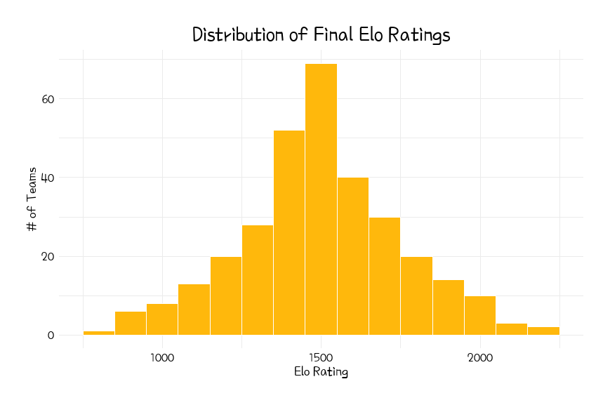
We can see that the final Elo ratings are somewhat normally distributed, ranging from below 1000 at the bottom end up to above 2000 for the absolute best teams as we saw above. In line with most Elo models, teams start with an intial Elo rating of 1500 which is also approximately at the centre of the distribution of teams' final Elo ratings.
Since we are only aiming to recreate an existing rating system here, this tutorial won't go too far into testing the Elo model's accuracy, but be aware that the elo package also includes some helpful helper functions for model evaluation, including Brier scores.
Using the Elo Model to Predict World Cup Results
Now that we have our Elo model and final team ratings, we can turn our attention toward future matches and making predictions using our ratings.
Start off by reading in the file.
## Rows: 544
## Columns: 6
## $ home_team <chr> "Qatar", "Senegal", "Qatar", "Netherlands", "Ecuador", …
## $ away_team <chr> "Ecuador", "Netherlands", "Senegal", "Ecuador", "Senega…
## $ stage <chr> "Group", "Group", "Group", "Group", "Group", "Group", "…
## $ home_team_prob <lgl> NA, NA, NA, NA, NA, NA, NA, NA, NA, NA, NA, NA, NA, NA,…
## $ draw_prob <dbl> NA, NA, NA, NA, NA, NA, NA, NA, NA, NA, NA, NA, NA, NA,…
## $ away_team_prob <lgl> NA, NA, NA, NA, NA, NA, NA, NA, NA, NA, NA, NA, NA, NA,…
We have information relating to the teams playing and the stage of the World Cup tournament during which the match will be played - now all we need to do is fill in the "home_team_prob", "draw_prob" and "away_team_prob" columns with the relevant probabilities using predictions based on our Elo ratings.
Accounting for Draws
Here is where things get a touch messy - Elo systems were originally devised to accommodate for two-player games of chess where winning or losing were the only two outcomes possible. For the group stage of the World Cup, drawn matches are also a possible outcome which means we need to accommodate for this in our predictions.
While there is no particularly obvious way to go about this, we can make do by using our historical match data to see how often teams draw for various Elo rating matchups. For example, at what rate does a team with a 400 Elo-point advantage draw with their opponent? In this instance, a 400 point advantage would see the better ranked team have a 91% chance of winning, but we would need to adjust that probability to include for a third possible outcome - the draw.
Let's find the draw rates for various differentials in win probability.
# Start by taking our Elo model, wrangling the match-by-match rating updates within the stored model and joining to our historic data set.
elo_results <- elo_model %>%
as_tibble() %>%
mutate(match_id = row_number()) %>%
select(match_id,
home_update = update.A,
away_update = update.B,
home_elo = elo.A,
away_elo = elo.B) %>%
# Join onto our historic data set using the match_id columns we created as a join key
right_join(final_dataset, by = "match_id")
We can now find the home and away win probabilities for each historic match and bucket them into groups at 5% increments according to how close the home and away win probabilities were. E.g. a team with a 90% chance to win coming up against a team with a 10% chance to win would have a 80% differential in win probability.
draw_rates <- elo_results %>%
mutate(home_elo_pre_match = home_elo - home_update,
away_elo_pre_match = away_elo - away_update,
home_prob = elo.prob(home_elo_pre_match, away_elo_pre_match),
away_prob = 1 - home_prob,
prob_diff = abs(home_prob - away_prob),
prob_diff_bucket = round(20*prob_diff)/20) %>% # Bucket into 20 groups at 5% increments between 0% and 100%
filter(year(date) >= 2005) %>% # Filter down to the past 15 years to only bucket matches once some fairly decent Elo ratings have been established
group_by(prob_diff_bucket) %>%
summarise(draw_rate = sum(home_result == 0.5)/n())
draw_rates %>% slice_head(n = 10)
## # A tibble: 10 × 2
## prob_diff_bucket draw_rate
## <dbl> <dbl>
## 1 0 0.320
## 2 0.05 0.296
## 3 0.1 0.289
## 4 0.15 0.271
## 5 0.2 0.285
## 6 0.25 0.256
## 7 0.3 0.273
## 8 0.35 0.270
## 9 0.4 0.276
## 10 0.45 0.240
We can visualise the draw rates for win probability differentials to get a better idea of how often draws happen in various scenarios.
draw_rates %>%
mutate(draw_rate = percent(draw_rate, digits = 0),
prob_diff_bucket = percent(prob_diff_bucket, digits = 0)) %>%
ggplot(aes(x = prob_diff_bucket, y = draw_rate)) +
geom_col(fill = "#ffb80c") +
geom_text(aes(label = draw_rate, y = draw_rate + 0.01),
size = 3.5, family = "poor_story") +
theme_minimal() +
scale_y_continuous(labels = scales::percent) +
scale_x_continuous(labels = scales::percent, breaks = scales::pretty_breaks()) +
labs(y = "Historic Draw Rate",
x = "Difference in Win Probability Between Home & Away Sides",
title = "Draw Frequency by Heaviness of Favouritism") +
theme(panel.background = element_rect(fill = "transparent", colour = NA),
plot.background = element_rect(fill = "transparent", colour = NA),
text = element_text(color = "black", family = "poor_story"),
axis.text = element_text(color = "black", size = 12),
plot.title = element_text(color = "black", size = 24, hjust = 0.5),
axis.title = element_text(family = "poor_story", size = 16),
plot.margin = unit(c(1,1,1,1), "cm"))
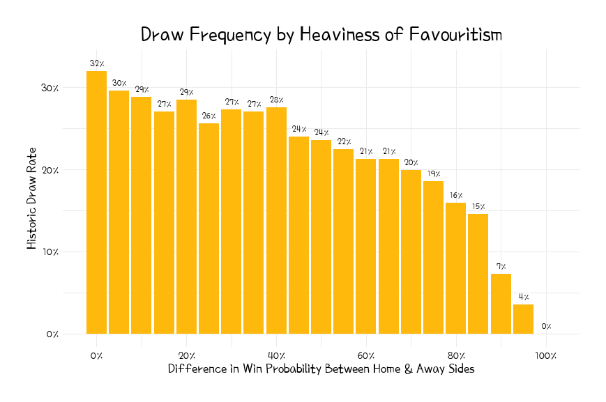
We can see that draws happen in more than 30% of matches where there has been a ~0% difference in win probability between the two sides (i.e. it was very close to a 50-50 match-up) - this is the highest draw rate, as one would expect. The draw rate falls away from there, to the point where only 3.5% of matches with a 95% win probability differential end in draws. Applying these draw rates to our group stage fixture predictions should allow for our Elo model to overcome the three-outcome nature of football.
Visualising Elo Ratings Through Time
Something we can do to help us better understand how the Elo model develops final team ratings is to visualise how a team's rating has developed over time. We know that the rating system dictates that all teams start with an initial rating of 1500, so we should expect to see teams move upward or down from there as a starting point depending on their fortunes.
Let's look at how Australia's Elo rating has changed through time.
elo_results %>%
select(match_id, date, home_team, home_elo) %>% rename(team = home_team, elo = home_elo) %>%
bind_rows(elo_results %>% select(match_id, date, away_team, away_elo) %>% rename(team = away_team, elo = away_elo)) %>%
arrange(match_id) %>%
filter(team == "Australia") %>%
ggplot(aes(x = date, y = elo, group = 1)) +
geom_hline(yintercept = 1500, linetype = "dashed", color = "black") +
geom_line(color = "#ffb80c", size = 1) +
theme_minimal() +
labs(x = "Year", y = "Elo Rating",
title = "Australia's Historic Elo Rating") +
theme(panel.background = element_rect(fill = "transparent", colour = NA),
plot.background = element_rect(fill = "transparent", colour = NA),
text = element_text(color = "black", family = "poor_story"),
axis.text = element_text(color = "black", size = 12),
plot.title = element_text(color = "black", size = 24, hjust = 0.5),
axis.title = element_text(family = "poor_story", size = 16),
plot.margin = unit(c(1,1,1,1), "cm"))
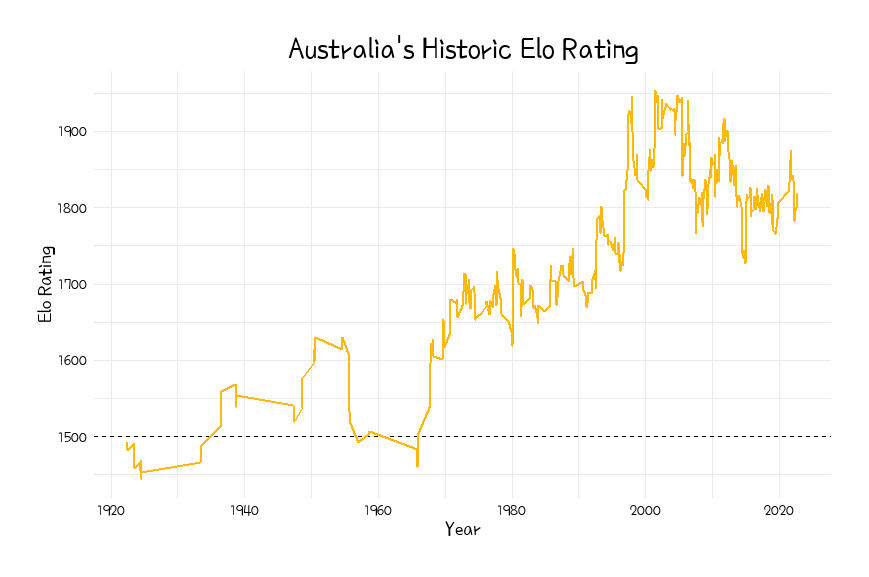
After a slow few decades initially with very few matches played, the Socceroos' Elo eventuall reached a peak rating of 1954 in June of 2001 (after a win against New Zealand) and has now settled back in the low-1800s range as of late 2022.
Making Predictions
Time to get back to making predictions - again using the elo package, the elo.calc() function can be used here to find the probability that a team with rating X will beat a team with rating Y.
From there we can overlay our draw rates and adjust as necessary to ensure all outcomes sum to equal 100%.
world_cup_predictions <- world_cup_matchups %>%
# Join on final home and away team Elo ratings ahead of calculating win probabilities
left_join(final_elos %>% rename(home_elo = elo), by = c("home_team" = "team")) %>%
left_join(final_elos %>% rename(away_elo = elo), by = c("away_team" = "team")) %>%
# Calculate win probabilities
mutate(home_team_prob = elo.prob(home_elo, away_elo),
away_team_prob = elo.prob(away_elo, home_elo),
# Just as we did with finding draw rates, group each match into probability differential buckets so that we can apply the correct draw rate
prob_diff = abs(home_team_prob - away_team_prob),
prob_diff_bucket = round(20*prob_diff)/20) %>%
# Join on our draw rates data frame - this essentially gives us the historic draw rate for the given match-up's probability split
left_join(draw_rates, by = "prob_diff_bucket") %>%
# update the draw_prob column accordingly for group stage matches. Set draw_prob to 0 for knockout matches where draws aren't possible.
mutate(draw_prob = case_when(stage == "Group" ~ draw_rate,
stage == "Knockout" ~ 0),
# Adjust home_team_prob and away_team_prob columns proportionally to allow for draw probability
home_team_prob = home_team_prob * (1 - draw_prob),
away_team_prob = away_team_prob * (1 - draw_prob)) %>%
# Remove redundant columns
select(home_team:away_team_prob)
# View 5 group stage matches and 5 knockout matches
world_cup_predictions %>% group_by(stage) %>% slice_head(n = 5)
model_name = "Elo_Tutorial"
file_name=paste(model_name,"_submission_file.csv",sep="")
write.csv(world_cup_predictions,file_name)
## # A tibble: 10 × 6
## # Groups: stage [2]
## home_team away_team stage home_team_prob draw_prob away_team_prob
## <chr> <chr> <chr> <dbl> <dbl> <dbl>
## 1 Qatar Ecuador Group 0.209 0.276 0.515
## 2 Senegal Netherlands Group 0.155 0.213 0.632
## 3 Qatar Senegal Group 0.276 0.256 0.468
## 4 Netherlands Ecuador Group 0.560 0.240 0.199
## 5 Ecuador Senegal Group 0.424 0.285 0.291
## 6 Qatar Senegal Knockout 0.371 0 0.629
## 7 Qatar Netherlands Knockout 0.126 0 0.874
## 8 Qatar Ecuador Knockout 0.289 0 0.711
## 9 Qatar England Knockout 0.218 0 0.782
## 10 Qatar USA Knockout 0.321 0 0.679
And there you have it - we've successfully created a model for predicting future match outcomes for the 2022 FIFA World Cup!
We hope you've found this tutorial useful - if you have any questions regarding predictive data modelling please reach out to automation@betfair.com.au.
Disclaimer
Note that whilst models and automated strategies are fun and rewarding to create, we can't promise that your model or betting strategy will be profitable, and we make no representations in relation to the code shared or information on this page. If you're using this code or implementing your own strategies, you do so entirely at your own risk and you are responsible for any winnings/losses incurred. Under no circumstances will Betfair be liable for any loss or damage you suffer.
Complete Code
packages <- c("tidyverse", "elo", "formattable", "lubridate", "showtext")
install.packages(setdiff(packages, rownames(installed.packages())))
library(tidyverse)
library(formattable)
library(elo)
library(lubridate)
library(showtext)
match_results <- read_csv("results.csv")
match_results %>% glimpse
match_results_wrangled <- match_results %>%
# Rename United States and South Korea to USA and Korea Republic respectively to reflect current naming. We need to do this to both 'home_team' and 'away_team' columns
mutate(home_team = case_when(home_team == "United States" ~ "USA",
home_team == "South Korea" ~ "Korea Republic",
TRUE ~ home_team),
away_team = case_when(away_team == "United States" ~ "USA",
away_team == "South Korea" ~ "Korea Republic",
TRUE ~ away_team),
# Add a new column for match result from both the home team and away team's perspectives. 1 = Win, 0.5 = Draw, 0 = Loss.
home_result = case_when(home_score > away_score ~ 1,
home_score < away_score ~ 0,
home_score == away_score ~ 0.5),
away_result = case_when(home_score < away_score ~ 1,
home_score > away_score ~ 0,
home_score == away_score ~ 0.5),
# Add a margin feature
margin = abs(home_score - away_score)) %>%
# If there are any matches missing score data, we don't want to use them for our Elo model - drop any data where we are missing a match margin
drop_na(margin)
final_dataset <- match_results_wrangled %>%
# Add a column to show 100 where there is a home ground advantage or 0 when played at a neutral venue. Our Elo model will call on this column for HGA.
mutate(hga = 100*!neutral,
# Allocate each tournament within the data to a K-weighting according to the above definition. Note that this section is quite open to interpretation.
tournament_weight = case_when(tournament == "FIFA World Cup" ~ 60,
tournament %in% c("Confederations Cup", "African Cup of Nations", "Copa América",
"UEFA Euro", "AFC Asian Cup") ~ 50,
str_detect(tolower(tournament), "qualification") ~ 40,
str_detect(tolower(tournament), " cup") ~ 40,
tournament %in% c("UEFA Nations League", "CONCACAF Nations League") ~ 40,
tournament == "Friendly" ~ 20,
TRUE ~ 30),
# Use our 'margin' feature to create the goal difference K-multiplier.
goal_diff_multiplier = case_when(margin <= 1 ~ 1,
margin == 2 ~ 1.5,
margin == 3 ~ 1.75,
margin >= 4 ~ 1.75 + (margin-3)/8),
# Combine the tournament weight and goal difference features to obtain our final K value for each match.
k = tournament_weight*goal_diff_multiplier,
# Also add a 'match_id' feaature to identify each match by number - we'll use this later.
match_id = row_number()) %>%
relocate(match_id)
elo_model <- elo.run(data = final_dataset,
formula = home_result ~ adjust(home_team, hga) + away_team + k(k))
final_elos <- final.elos(elo_model) %>%
enframe(name = "team", value = "elo") %>%
arrange(desc(elo))
# See the top 10 rated nations
final_elos %>% slice_head(n = 10)
# Load Google fonts from https://fonts.google.com/
font_add_google(name = "Poor Story", family = "poor_story")
showtext_auto()
# Visualise final Elo ratings
final_elos %>%
ggplot(aes(x = elo)) +
geom_histogram(binwidth = 100, fill = "#ffb80c", color = "white") +
theme_minimal() +
labs(x = "Elo Rating",
y = "# of Teams",
title = "Distribution of Final Elo Ratings") +
theme(panel.background = element_rect(fill = "transparent", colour = NA),
plot.background = element_rect(fill = "transparent", colour = NA),
text = element_text(color = "black", family = "poor_story"),
axis.text = element_text(color = "black", size = 14),
plot.title = element_text(color = "black", size = 24, hjust = 0.5),
axis.title = element_text(family = "poor_story", size = 16),
plot.margin = unit(c(1,1,1,1), "cm"))
brier(elo_model)
world_cup_matchups <- read_csv("dummy_submission_file.csv")

world_cup_matchups %>% glimpse
# Start by taking our Elo model, wrangling the match-by-match rating updates within the stored model and joining to our historic data set.
elo_results <- elo_model %>%
  as_tibble() %>%
  mutate(match_id = row_number()) %>%
  select(match_id,
         home_update = update.A,
         away_update = update.B,
         home_elo = elo.A,
         away_elo = elo.B) %>%

  # Join onto our historic data set using the match_id columns we created as a join key
  right_join(final_dataset, by = "match_id")
draw_rates <- elo_results %>%
  mutate(home_elo_pre_match = home_elo - home_update,
         away_elo_pre_match = away_elo - away_update,
         home_prob = elo.prob(home_elo_pre_match, away_elo_pre_match),
         away_prob = 1 - home_prob,
         prob_diff = abs(home_prob - away_prob),
         prob_diff_bucket = round(20*prob_diff)/20) %>% # Bucket into 20 groups at 5% increments between 0% and 100%
  filter(year(date) >= 2005) %>%  # Filter down to the past 15 years to only bucket matches once some fairly decent Elo ratings have been established
  group_by(prob_diff_bucket) %>%
  summarise(draw_rate = sum(home_result == 0.5)/n())

draw_rates %>% slice_head(n = 10)
draw_rates %>%
  mutate(draw_rate = percent(draw_rate, digits = 0),
         prob_diff_bucket = percent(prob_diff_bucket, digits = 0)) %>%
  ggplot(aes(x = prob_diff_bucket, y = draw_rate)) +
  geom_col(fill = "#ffb80c") +
  geom_text(aes(label = draw_rate, y = draw_rate + 0.01),
            size = 3.5, family = "poor_story") +
  theme_minimal() +
  scale_y_continuous(labels = scales::percent) +
  scale_x_continuous(labels = scales::percent, breaks = scales::pretty_breaks()) +
  labs(y = "Historic Draw Rate",
       x = "Difference in Win Probability Between Home & Away Sides",
       title = "Draw Frequency by Heaviness of Favouritism") +
  theme(panel.background = element_rect(fill = "transparent", colour = NA),
        plot.background = element_rect(fill = "transparent", colour = NA),
        text = element_text(color = "black", family = "poor_story"),
        axis.text = element_text(color = "black", size = 12),
        plot.title = element_text(color = "black", size = 24, hjust = 0.5),
        axis.title = element_text(family = "poor_story", size = 16),
        plot.margin = unit(c(1,1,1,1), "cm"))
elo_results %>%
  select(match_id, date, home_team, home_elo) %>% rename(team = home_team, elo = home_elo) %>%
  bind_rows(elo_results %>% select(match_id, date, away_team, away_elo) %>% rename(team = away_team, elo = away_elo)) %>%
  arrange(match_id) %>%
  filter(team == "Australia") %>%
  ggplot(aes(x = date, y = elo, group = 1)) +
  geom_hline(yintercept = 1500, linetype = "dashed", color = "black") +
  geom_line(color = "#ffb80c", size = 1) +
  theme_minimal() +
  labs(x = "Year", y = "Elo Rating",
       title = "Australia's Historic Elo Rating") +
  theme(panel.background = element_rect(fill = "transparent", colour = NA),
        plot.background = element_rect(fill = "transparent", colour = NA),
        text = element_text(color = "black", family = "poor_story"),
        axis.text = element_text(color = "black", size = 12),
        plot.title = element_text(color = "black", size = 24, hjust = 0.5),
        axis.title = element_text(family = "poor_story", size = 16),
        plot.margin = unit(c(1,1,1,1), "cm"))
world_cup_predictions <- world_cup_matchups %>%
  # Join on final home and away team Elo ratings ahead of calculating win probabilities
  left_join(final_elos %>% rename(home_elo = elo), by = c("home_team" = "team")) %>%
  left_join(final_elos %>% rename(away_elo = elo), by = c("away_team" = "team")) %>%

  # Calculate win probabilities
  mutate(home_team_prob = elo.prob(home_elo, away_elo),
         away_team_prob = elo.prob(away_elo, home_elo),

         # Just as we did with finding draw rates, group each match into probability differential buckets so that we can apply the correct draw rate
         prob_diff = abs(home_team_prob - away_team_prob),
         prob_diff_bucket = round(20*prob_diff)/20) %>%

  # Join on our draw rates data frame - this essentially gives us the historic draw rate for the given match-up's probability split
  left_join(draw_rates, by = "prob_diff_bucket") %>%

  # update the draw_prob column accordingly for group stage matches. Set draw_prob to 0 for knockout matches where draws aren't possible.
  mutate(draw_prob = case_when(stage == "Group" ~ draw_rate,
                               stage == "Knockout" ~ 0),

         # Adjust home_team_prob and away_team_prob columns proportionally to allow for draw probability
         home_team_prob = home_team_prob * (1 - draw_prob),
         away_team_prob = away_team_prob * (1 - draw_prob)) %>%

  # Remove redundant columns
  select(home_team:away_team_prob)

# View 5 group stage matches and 5 knockout matches
world_cup_predictions %>% group_by(stage) %>% slice_head(n = 5)

model_name = "Elo_Tutorial"
file_name=paste(model_name,"_submission_file.csv",sep="")
write.csv(world_cup_predictions,file_name)