Automated betting angles in Python
| Betting strategies based on your existing insights: no modelling required
Workshop
This tutorial was written by Tom Bishop and was originally published on Github. It is shared here with his permission.
This tutorial follows on logically from the JSON to CSV tutorial and backteseting ratings in Python tutorial we shared previously. If you're still new to working with the JSON data sets we suggest you take a look at those tutorials before diving into this one.
As always please reach out with feedback, suggestions or queries, or feel free to submit a pull request if you catch some bugs or have other improvements!
This article was written more than 2 years ago and some packages used here will have changed since the article was written. Continue at your peril
Cheat sheet
- This is presented as a Jupyter notebook as this format is interactive and lets you run snippets of code from wihtin the notebook. To use this functionality you'll need to download a copy of the
ipynbfile locally and open it in a text editor (i.e. VS code). - If you're looking for the complete code head to the bottom of the page or download the script from Github.
- To run the code, save it to your machine, open a command prompt, or a terminal in your text editor of choice (we're using VS code), make sure you've navigated in the terminal to the folder you've saved the script in and then type
py main.py(or whatever you've called your script file if not main) then hit enter. To stop the code running use Ctrl C. - Make sure you amend your data path to point to your data file. We'll be taking in an input of a historical tar file downloaded from the Betfair historic data site. We're using a PRO version, though the code should work on ADVANCED too. This approach won't work with the BASIC data tier.
- We're using the
betfairlightweightpackage to do the heavy lifting - We've also posted the completed code logic on the
betfair-downunderGithub repo.
0.1 Setup
Once again I'll be presenting the analysis in a jupyter notebook and will be using python as a programming language.
Some of the data processing code takes a while to execute - that code will be in cells that are commented out - and will require a bit of adjustment to point to places on your computer where you want to locally store the intermediate data files.
You'll also need betfairlightweight which you can install with something like pip install betfairlightweight.
import requests
import pandas as pd
from datetime import date, timedelta
import numpy as np
import os
import re
import tarfile
import zipfile
import bz2
import glob
import logging
import yaml
from unittest.mock import patch
from typing import List, Set, Dict, Tuple, Optional
from itertools import zip_longest
import betfairlightweight
from betfairlightweight import StreamListener
from betfairlightweight.resources.bettingresources import (
    PriceSize,
    MarketBook
)
from scipy.stats import t
import plotly.express as px
0.2 Context
Formulating betting angles (or "strategies" as some call them) is quite a common pasttime for some. These angles can range all the way from very simple to quite sophisticated, and could include things like:
- Laying NBA teams playing on the second night of a back-to-back
- Laying AFL team coming off a bye when matched against a team who played last week
- Backing a greyhound in boxes 1 or 2 in short sprint style races
- Backing a horse pre-race who typically runs at the front of the field and placing an order to lay the same horse if it shortens to some lower price in-play, locking in a profit
Beyond the complexity of the actual concept what really seperates these angles is evidence. You might have heard TV personalities and betting ads suggest a certain strategy (resembling one of the above) are real-world predictive trends but they rarely are. They are rarely derived from the right historical data or are concluded without the necessary statistical rigour. Most simply formulated their angles off intuition or observing a trend across a small sample of data.
There are many users on betting exchanges who profit off these angles. In fact, when most people talk about automated or sophisticated exchange betting they are often talking about automating these kind of betting angles, as opposed to betting ratings produced from a sophisticated bottom-up fundemental modelling. That's because profitable fundemental modelling (where your model which arrives at some estimation of fair value from first principles) is very hard.
The reason this approach is so much easier is that you assume the market odds are right except x and go from there, applying small top-down adjustments for factors that haven't historically been incorporated in the market opinion. The challenge lies in finding those factors and making sure you aren't tricking yourself in thinking you've found one that you can profit off in the future.
Once again this is another example of the uses of the Betfair historical stream data. To get cracking - as always - we need historical odds and the best place to get that is to self serve the historical stream files.
0.3 Examples
I'll go through an end-to-end example of 3 different betting angles on Australian thoroughbred racing. Which will include: Which will include:
- Sourcing data
- Assembling data
- Formulating hypotheses
- Testing Hypotheses
- Discussion about implementation
1.0 Data
1.1 Betfair Odds Data
We'll follow a very similar template as other tutorials extracting key information from the betfair stream data.
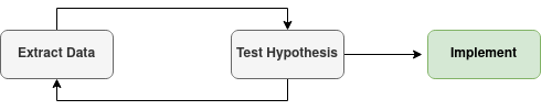
It's important to note that given the volume of data you need to handle with these stream files, your workflow will probably involve choosing some methods of aggregation / summary that you'll reconsider after your first cut of analysis. Parsing and saving a dataset, using it to test some hypotheses which likely results in more questions that need to be examined by reparsing the stream files in a slightly different way. Your workflow will likely follow something like this diagram.
For the purposes of this article I'm interested in backtesting some betting angles at the BSP, using some indication of price momentum/market support in some angles, and testing some back to lay strategies so we'll need to pull out some information about each runners in-play trading.
So we'll extract the following for each runner: - BSP - Last Traded Price - Volume Weighted Avg Price (top 3 boxes) 5 mins before the scheduled jump time - Volume Weighted Avg Price (top 3 boxes) 30 seconds before the scheduled jump time - The volume traded on the selection - The minimum "best available to lay" price offered inplay (which is a measure of how low the selection traded during the race)
First we'll establish some utility functions needed to parse the data. Most of these were discussed in the previous backtest your ratings tutorial.
# Utility Functions For Stream Parsing
# _________________________________

def as_str(v) -> str:
    return '%.2f' % v if type(v) is float else v if type(v) is str else ''

def split_anz_horse_market_name(market_name: str) -> (str, str, str):
    parts = market_name.split(' ')
    race_no = parts[0] # return example R6
    race_len = parts[1] # return example 1400m
    race_type = parts[2].lower() # return example grp1, trot, pace
    return (race_no, race_len, race_type)

def filter_market(market: MarketBook) -> bool:
    d = market.market_definition
    return (d.country_code == 'AU'
        and d.market_type == 'WIN'
        and (c := split_anz_horse_market_name(d.name)[2]) != 'trot' and c != 'pace')

def load_markets(file_paths):
    for file_path in file_paths:
        print(file_path)
        if os.path.isdir(file_path):
            for path in glob.iglob(file_path + '**/**/*.bz2', recursive=True):
                f = bz2.BZ2File(path, 'rb')
                yield f
                f.close()
        elif os.path.isfile(file_path):
            ext = os.path.splitext(file_path)[1]
            # iterate through a tar archive
            if ext == '.tar':
                with tarfile.TarFile(file_path) as archive:
                    for file in archive:
                        yield bz2.open(archive.extractfile(file))
            # or a zip archive
            elif ext == '.zip':
                with zipfile.ZipFile(file_path) as archive:
                    for file in archive.namelist():
                        yield bz2.open(archive.open(file))

    return None

def slicePrice(l, n):
    try:
        x = l[n].price
    except:
        x = np.nan
    return(x)

def sliceSize(l, n):
    try:
        x = l[n].size
    except:
        x = np.nan
    return(x)

def wapPrice(l, n):
    try:
        x = round(sum( [rung.price * rung.size for rung in l[0:(n-1)] ] ) / sum( [rung.size for rung in l[0:(n-1)] ]),2)
    except:
        x = np.nan
    return(x)

def ladder_traded_volume(ladder):
    return(sum([rung.size for rung in ladder]))
Then we'll create our core execution functions that will scan over the historical stream files and use betfairlightweight to recreate the state of the exchange for each thoroughbred market and extract key information for each selection
# Core Execution Fucntions
# _________________________________

def extract_components_from_stream(s):

    with patch("builtins.open", lambda f, _: f):

        evaluate_market = None
        prev_market = None
        postplay = None
        preplay = None
        t5m = None
        t30s = None
        inplay_min_lay = None

        gen = s.get_generator()

        for market_books in gen():

            for market_book in market_books:

                # If markets don't meet filter return None's
                if evaluate_market is None and ((evaluate_market := filter_market(market_book)) == False):
                    return (None, None, None, None, None, None)

                # final market view before market goes in play
                if prev_market is not None and prev_market.inplay != market_book.inplay:
                    preplay = market_book

                # final market view before market goes is closed for settlement
                if prev_market is not None and prev_market.status == "OPEN" and market_book.status != prev_market.status:
                    postplay = market_book

                # Calculate Seconds Till Scheduled Market Start Time
                seconds_to_start = (market_book.market_definition.market_time - market_book.publish_time).total_seconds()

                # Market at 30 seconds before scheduled off
                if t30s is None and seconds_to_start < 30:
                    t30s = market_book

                # Market at 5 mins before scheduled off
                if t5m is None and seconds_to_start < 5*60:
                    t5m = market_book

                # Manage Inplay Vectors
                if market_book.inplay:

                    if inplay_min_lay is None:
                        inplay_min_lay = [ slicePrice(runner.ex.available_to_lay,0) for runner in market_book.runners]
                    else:
                        inplay_min_lay = np.fmin(inplay_min_lay, [ slicePrice(runner.ex.available_to_lay,0) for runner in market_book.runners])

                # update reference to previous market
                prev_market = market_book

        # If market didn't go inplay
        if postplay is not None and preplay is None:
            preplay = postplay
            inplay_min_lay = ["" for runner in market_book.runners]

        return (t5m, t30s, preplay, postplay, inplay_min_lay, prev_market) # Final market is last prev_market

def parse_stream(stream_files, output_file):

    with open(output_file, "w+") as output:

        output.write("market_id,selection_id,selection_name,wap_5m,wap_30s,bsp,ltp,traded_vol,inplay_min_lay\n")

        for file_obj in load_markets(stream_files):

            stream = trading.streaming.create_historical_generator_stream(
                file_path=file_obj,
                listener=listener,
            )

            (t5m, t30s, preplay, postplay, inplayMin, final) = extract_components_from_stream(stream)

            # If no price data for market don't write to file
            if postplay is None or final is None or t30s is None:
                continue;

            # All runner removed
            if all(runner.status == "REMOVED" for runner in final.runners):
                continue

            runnerMeta = [
                {
                    'selection_id': r.selection_id,
                    'selection_name': next((rd.name for rd in final.market_definition.runners if rd.selection_id == r.selection_id), None),
                    'selection_status': r.status,
                    'sp': r.sp.actual_sp
                }
                for r in final.runners
            ]

            ltp = [runner.last_price_traded for runner in preplay.runners]

            tradedVol = [ ladder_traded_volume(runner.ex.traded_volume) for runner in postplay.runners ]

            wapBack30s = [ wapPrice(runner.ex.available_to_back, 3) for runner in t30s.runners]

            wapBack5m = [ wapPrice(runner.ex.available_to_back, 3) for runner in t5m.runners]

            # Writing To CSV
            # ______________________

            for (runnerMeta, ltp, tradedVol, inplayMin, wapBack5m, wapBack30s) in zip(runnerMeta, ltp, tradedVol, inplayMin, wapBack5m, wapBack30s):

                if runnerMeta['selection_status'] != 'REMOVED':

                    output.write(
                        "{},{},{},{},{},{},{},{},{}\n".format(
                            str(final.market_id),
                            runnerMeta['selection_id'],
                            runnerMeta['selection_name'],
                            wapBack5m,
                            wapBack30s,
                            runnerMeta['sp'],
                            ltp,
                            round(tradedVol),
                            inplayMin
                        )
                    )
Finally, after sourcing and downloading 12 months of stream files (ask automation@betfair.com.au for more info if you don't know how to do this) we'll use the above code to parse each file and write to a single csv file to be used for analysis.
# Description:
#   Will loop through a set of stream data archive files and extract a few key pricing measures for each selection
# Estimated Time:
#   ~6 hours

# Parameters
# _________________________________

# trading = betfairlightweight.APIClient("username", "password")

# listener = StreamListener(max_latency=None)

# stream_files = glob.glob("[PATH TO LOCAL FOLDER STORING ARCHIVE FILES]*.tar")
# output_file = "[SOME OUTPUT DIRECTORY]/thoroughbred-odds-2021.csv"

# Run
# _________________________________

# if __name__ == '__main__':
#     parse_stream(stream_files, output_file)
1.2 Race Data
If you're building a fundamental bottom-up model, finding and managing ETL from an appropriate data source is a large part of the exercise. If your needs are simpler (for these types of automated strategies for example) there's plenty of good information that's available right inside the betfair API itself.
The RUNNER_METADATA slot inside the listMarketCatalogue response for example will return a pretty good slice of metadata about the horses racing in upcoming races including but not limited to: the trainer, the jockey, the horses age, and a class rating. The documentaion for this endpoint will give you the full extent of this what's inside this response.
Our problem for this exercise is that the historical stream files don't include this RUNNER_METADATA so we weren't able to extract it in the previous step. However, a sneaky workaround is to use an unsuppoerted back-end endpoint, one which Betfair use for the Hub racing results page.
These API endpoints are:
- Market result data: https://apigateway.betfair.com.au/hub/raceevent/1.154620281
- Day’s markets: https://apigateway.betfair.com.au/hub/racecard?date=2018-12-18
Extract Betfair Racing Markets for a Given Date
First we'll hit the https://apigateway.betfair.com.au/hub/racecard endpoint to get the racing markets available on Betfair for a given day in the past:
def getBfMarkets(dte):

    url = 'https://apigateway.betfair.com.au/hub/racecard?date={}'.format(dte)

    responseJson = requests.get(url).json()

    marketList = []

    for meeting in responseJson['MEETINGS']:
        for markets in meeting['MARKETS']:
            marketList.append(
                {
                    'date': dte,
                    'track': meeting['VENUE_NAME'],
                    'country': meeting['COUNTRY'],
                    'race_type': meeting['RACE_TYPE'],
                    'race_number': markets['RACE_NO'],
                    'market_id': str('1.' + markets['MARKET_ID']),
                    'start_time': markets['START_TIME']
                }
            )

    marketDf = pd.DataFrame(marketList)

    return(marketDf)
Extract Key Race Metadata
Then (for one of these market_ids) we'll hit the https://apigateway.betfair.com.au/hub/raceevent/ enpdoint to get some key runner metadata for the runners in this race. It's important to note that this information is available through the Betfair API so we won't need to go to a secondary datasource to find it at the point of implementation, this would add a large layer of complexity to the project including things like string cleaning and matching.
def getBfRaceMeta(market_id):

    url = 'https://apigateway.betfair.com.au/hub/raceevent/{}'.format(market_id)

    responseJson = requests.get(url).json()

    if 'error' in responseJson:
        return(pd.DataFrame())

    raceList = []

    for runner in responseJson['runners']:

        if 'isScratched' in runner and runner['isScratched']:
            continue

        # Jockey not always populated
        try:
            jockey = runner['jockeyName']
        except:
            jockey = ""

        # Place not always populated
        try:
            placeResult = runner['placedResult']
        except:
            placeResult = ""

        # Place not always populated
        try:
            trainer = runner['trainerName']
        except:
            trainer = ""

        raceList.append(
            {
                'market_id': market_id,
                'weather': responseJson['weather'],
                'track_condition': responseJson['trackCondition'],
                'race_distance': responseJson['raceLength'],
                'selection_id': runner['selectionId'],
                'selection_name': runner['runnerName'],
                'barrier': runner['barrierNo'],
                'place': placeResult,
                'trainer': trainer,
                'jockey': jockey,
                'weight': runner['weight']
            }
        )

    raceDf = pd.DataFrame(raceList)

    return(raceDf)
Wrapper Function
Stiching these two functions together we can create a wrapper function that hits both endpoints for all the thoroughbred races in a given day and extract all the runner metadata and results.
def scrapeThoroughbredBfDate(dte):

    markets = getBfMarkets(dte)

    if markets.shape[0] == 0:
        return(pd.DataFrame())

    thoMarkets = markets.query('country == "AUS" and race_type == "R"')

    if thoMarkets.shape[0] == 0:
        return(pd.DataFrame())

    raceMetaList = []

    for market in thoMarkets.market_id:
        raceMetaList.append(getBfRaceMeta(market))

    raceMeta = pd.concat(raceMetaList)

    return(markets.merge(raceMeta, on = 'market_id'))
Then to produce a historical slice of all races between two dates we could just loop over a set of dates and append each results set
# Description:
#   Will loop through a set of dates (starting July 2020 in this instance) and return race metadata from betfair
# Estimated Time:
#   ~60 mins
#
# dataList = []
# dateList = pd.date_range(date(2020,7,1),date.today()-timedelta(days=1),freq='d')
# for dte in dateList:
#     dte = dte.date()
#     print(dte)
#     races = scrapeThoroughbredBfDate(dte)
#     dataList.append(races)
# data = pd.concat(dataList)
# data.to_csv("[LOCAL PATH SOMEWHERE]", index=False)
2.0 Analysis
I'll be running through 3 simple betting angles, one easy, one medium, and one hard to illustrate different types of angles you might want to try at home. The process I lay out is very similar (if not identical) but the implementation might be a bit trickier in each case and might take a little more programming skill to get up and running.
We'll use a simple evaluation function (POT and strike rate) to evaluate each of these strategies.
2.1 Assemble Data
Now that we have our 2 core datasets (odds + race / runner metadata) we can join them together and do some analysis
# Local Paths (will be different on your machine)
path_odds_local = "[PATH TO YOUR LOCAL FILES]/thoroughbred-odds-2021.csv"
path_race_local = "[PATH TO YOUR LOCAL FILES]/thoroughbred-race-data.csv"
odds = pd.read_csv(path_odds_local, dtype={'market_id': object, 'selection_id': object})
race = pd.read_csv(path_race_local, dtype={'market_id': object, 'selection_id': object})
2.2 Methodology
Looping back around to the context discussion in part 0.2 we need to decide on how to set up our analysis that will help us: find angles, formulate strategies, and test them with enough rigour that will give us a good estimate of our forward looking profitability on any that we choose to implement and automate.
The 3 key tricks I'll lay out in this piece are: - Using a statistical estimate to quantify the robustness of historical profitibalility - Using out-of-sample validation (much like a you would in a model building exercise) to get an accurate view of forward looking profitability - Using domain knowledge to chunk selections to get broader sample for more stable estimate of profitability
2.3.1 Chunking
This is a technique you can use to group together variables in conceptually similar groups. For example, thoroughbred races are run over many different exact distances (800m, 810m, 850m, 860m etc) which - using a domain overlay - are all very short sprint style races for a horse race. Similarly, barriers 1, 2 and 3 being on the very inside of the race field and closest to the rail all present similar early race challenges and advantages for horses jumping from those barriers.
So formulating your betting angles you may want to overlay semantically similar variable groups to test your betting hypothesis.
I'll add variable chunks for race distance and barrier for now but you may want to test more (for example horse experience, trainer stable size etc)
def distance_group(distance):
if distance is None:
return("missing")
elif distance < 1100:
return("sprint")
elif distance < 1400:
return("mid_short")
elif distance < 1800:
return("mid_long")
else:
return("long")
def barrier_group(barrier):
if barrier is None:
return("missing")
elif barrier < 4:
return("inside")
elif barrier < 9:
return("mid_field")
else:
return("outside")
df['distance_group'] = pd.to_numeric(df.race_distance, errors = "coerce").apply(distance_group)
df['barrier_group'] = pd.to_numeric(df.barrier, errors = "coerce").apply(barrier_group)
2.3.2 In Sample vs Out of Sample
The first thing I'm going to do is to split off a largish chunk of my data before even looking at it. I'll ultimately use it to paper trade some of my candidate angles but I want it to be as seperate from the idea generation process as possible.
I'll use the model building nomenclature "train" and "test" even though I'm not really doing any "training". My data contains all AUS thoroughbred races from July 2020 until end of June 2021 so I'll cut off the period Apr-June 2021 as my "test" set.
2.3.3 Statistically Measuring Profit
Betting outcomes, and the randomness associated with them, at their core are the types of things the discipline of statistics was created to solve. Concepts like sample size, expected value, and variance are terms you might hear from sophisticated (and some novice) bettors and they are all drawn from the field of statistics. Though you don't need to become a PHD of statistics every little extra technique or concept you can glean from the field will help your betting if you want it to.
To illustrate with an example, let's group by net backing profit on turnover for a horse to see which horses have the highest historical back POT:
So back Little Vulpine whenever it races? We all know intuitively what's wrong with that betting angle - it's raced one time in our sample and happened to win at a bsp of 270. Sample size and variance are dominating this simple measure of historical POT.
Instead what we can do is treat the historical betting outcomes as a random variable and apply some statistical tests of signifance to them. A more detailed discussion of this particular test can be found here as can an excel calculator you can input your stats into. I'll simply translate the test to python to enable it's use when formulating our betting angles.
The TLDR version of this test is that; based on your bet sample size, your profit, and the average odds across that sample of bets, the calculation produces a p value which estimates the probability your profit (or loss) happened by pure chance (where chance would be an expectation of breakeven betting simply at fair odds).
That doesn't mean we can formulate our angles and use this metric (and this metric alone) to validate their profitability. You'll find that it will give you misleading results in some instances. As analysts we're also prone to finding infinite different ways to unintentionally overfit our analysis as you might have heard elsewhere described as the concept of p-hacking, but it does give us an extra filter to cast over our hypotheses before really validating them with out-of-sample testing.
2.4 Angle 1: Track | Distance | Barrier
The first thing I'll test is whether or not there are any combinations of track/distance/barrier where backing or laying could produce robust long term profit. This probably fits within the types of betting angles people before you have already sucked all the value out of long before you started reading this article. That's not to say that you shouldn't test them though, as people have made livings on betting angles as simple as these.
# Calculate the profit (back and lay) and average odds across all track / distance / barrier group combos
trackDistanceBarrier = (
dfTrain
.assign(stake = 1)
.assign(odds = lambda x: x['bsp'])
.groupby(['track', 'race_distance', 'barrier_group'], as_index=False)
.agg({'back_npl': 'sum', 'lay_npl': 'sum','stake': 'sum', 'odds': 'mean'})
)
trackDistanceBarrier
So it looks like over 2 selections jumping from the inside 3 barriers at Albany 1000m you would have made a healthy profit if you'd decide to back them historically.
Let's use our lense of statistical significance to view these profit figures
trackDistanceBarrier = (
trackDistanceBarrier
.assign(backPL_pValue = lambda x: pl_pValue(number_bets = x['stake'], npl = x['back_npl'], stake = x['stake'], average_odds = x['odds']))
.assign(layPL_pValue = lambda x: pl_pValue(number_bets = x['stake'], npl = x['lay_npl'], stake = x['stake'], average_odds = x['odds']))
)
trackDistanceBarrier
So as you can see, whilst having a back POT of nearly 500% because the results were generated over 2 runners at quite high odds the p value (50%) suggest that it's quite likely we could have seen these exact results due to randomness, which is very intuitive.
Let's have a look to see if there's any statistically significant edge to be gained on the lay side
So despite high lay POT none of these angles suggest an irrefutablely profitable angle laying these combinations. However, that doesn't mean we shouldn't test them on our out of sample set of races. These are our statistically most promising examples, we'll just take the top 5 for now and see how we would have performed if we had of started betting them on April first 2021.
Keep in mind this should give us a pretty good indication of what we could get over the next 3 months into the future if we started today because we haven't contaminated/leaked any data from the post April period into our angle formulation.
# First let's test laying on the train set (by definition we know these will be profitable)
train_TDB_bestLay = (
dfTrain
.merge(TDB_bestLay[['track', 'race_distance']])
.assign(npl=lambda x: x['lay_npl'])
.assign(stake=1)
.assign(win=lambda x: np.where(x['lay_npl'] > 0, 1, 0))
)
# This is the key test (non of the races has been part of analysis to this point)
test_TDB_bestLay = (
dfTest
.merge(TDB_bestLay[['track', 'race_distance']])
.assign(npl=lambda x: x['lay_npl'])
.assign(stake=1)
.assign(win=lambda x: np.where(x['lay_npl'] > 0, 1, 0))
)
# Peaking at the bets in the test set
test_TDB_bestLay[['track', 'race_distance', 'barrier', 'barrier_group', 'bsp', 'lay_npl', 'win', 'stake']]
That's promising results. Our test set shows similar betting performance as our training set and we're still seeing a profitble trend. These are lay strategies so they aren't as robust as backing strategies as your profit distribution is lots of small wins and some large losses, but this is potentially a profitble betting angle!
2.5 Angle 2: Jockeys + Market Opinion
Moving up slightly in level of difficulty our angles could include different kinds of reference points. Jockeys seem to be a divisive form factor in thoroughbred racing, and their quality can be hard to isolate relative to the quality of the horse and its preperation etc.
I'm going to look at isolating jockeys that are either favoured or unfavoured by the market to see if I can formulate a betting angle that could generate me expected profit.
The metric I'm going to use to determine market favour will be the ratio between back price 5 minutes before the scheduled jump and 30 seconds before the scheduled jump. Plotting this ratio for jockeys in our training set we can see which jockeys tend to have high market support by a high ratio (horses they are riding tend to shorten before the off)
Next, let's split the sample of each jockey's races between two scenarios a) the market firmed for their horse b) their horse drifted in the market in the last 5 minutes of trading.
We then calculate the same summary table of inputs (profit, average odds etc) for backing these jockeys at the BSP given some market move. We can then feed these metrics into our statistical significance test to get an idea of the profitability of each combination.
# Group By Jockey and Market Support
jockeys = (
dfTrain
.assign(stake = 1)
.assign(odds = lambda x: x['bsp'])
.assign(npl=lambda x: np.where(x['place'] == 1, 0.95 * (x['odds']-1), -1))
.assign(market_support=lambda x: np.where(x['wap_5m'] > x['wap_30s'], "Y", "N"))
.groupby(['jockey', 'market_support'], as_index=False)
.agg({'odds': 'mean', 'stake': 'sum', 'npl': 'sum'})
.assign(pValue = lambda x: pl_pValue(number_bets = x['stake'], npl = x['npl'], stake = x['stake'], average_odds = x['odds']))
)
jockeys.sort_values('pValue').query('npl > 0').head(10)
You can think of each of these scenarios representing different cases. If profitable: - Under market support this could indicate the jockey is being correctly favoured to maximise their horse's chances of winning the race or perhaps even some kind of insider knowledge coming out of certain stables - Under market drift this could indicate some incorrect skepticism about the jockeys ability and thus their horse has been overlayed
Either way we're interested to see how these combinations would perform paper trading in our out of sample set
# First evaluate on our training set
train_jockeyMarket = (
dfTrain
.assign(market_support=lambda x: np.where(x['wap_5m'] > x['wap_30s'], "Y", "N"))
.merge(jockeys.sort_values('pValue').query('npl > 0').head(10)[['jockey', 'market_support']])
.assign(stake = 1)
.assign(odds = lambda x: x['bsp'])
.assign(npl=lambda x: np.where(x['place'] == 1, 0.95 * (x['odds']-1), -1))
.assign(win=lambda x: np.where(x['npl'] > 0, 1, 0))
)
# And on the test set
test_jockeyMarket = (
dfTest
.assign(market_support=lambda x: np.where(x['wap_5m'] > x['wap_30s'], "Y", "N"))
.merge(jockeys.sort_values('pValue').query('npl > 0').head(10)[['jockey', 'market_support']])
.assign(stake = 1)
.assign(odds = lambda x: x['bsp'])
.assign(npl=lambda x: np.where(x['place'] == 1, 0.95 * (x['odds']-1), -1))
.assign(win=lambda x: np.where(x['npl'] > 0, 1, 0))
)
You can see overfitting in full effect here with the train set performance. However, our out-of-sample performance is still decently profitable. We might have found another profitable betting angle!
It's worth noting that implementing this strategy would be slightly more complex than implementing our first strategy. Our code (or third party tool) would need to be able to check whether the market had firmed between 2 distinct time points before the jump of the race and cross reference that with the jockey name. Trivial for someone who is comfortable with bet placement and the betfair API but a little more involved for the uninitiated. It's important to formulate angles that you would know how and are capable of implementing.
2.6 Angle 3: Backing To Lay
Now let's try to use some of our inplay price data we extracted from the stream files. I'm interested in testing some back-to-lay strategies where a horse is backed preplay with the intention to get some tradeout lay order filled during the race. The types of scenarios where this could be conceivably profitable would be on certain kinds of horses or jockeys that show promise or strength early in the race but generally fade late and might not convert those early advantages often.
Things we could look at here are: - Horses that typically trade lower than their preplay odds but don't win often - Jockeys that typically trade lower than their preplay odds but don't win often - Certain combinations of jockey / trainer / horse / race distance that meet these criteria
# First Investigate The Average Inplay Minimums And Loss Rates of Certain Jockeys
tradeOutIndex = (
dfTrain
.query('distance_group in ["long", "mid_long"]')
.assign(inplay_odds_ratio=lambda x: x['inplay_min_lay'] / x['bsp'])
.assign(win=lambda x: np.where(x['place']==1,1,0))
.assign(races=lambda x: 1)
.groupby(['jockey'], as_index=False)
.agg({'inplay_odds_ratio': 'mean', 'win': 'mean', 'races': 'sum'})
.sort_values('inplay_odds_ratio')
.query('races >= 5')
)
tradeOutIndex
Ok so what we have here is a list of all jockeys with over 5 races on long and mid-long race distance groups (over 1800m) ordered by their average ratio of inplay minimum traded price compared with their jump price.
If this trend is predictive we could assume that these jockeys tend to have an agressive race style and like to get out and lead the race. We'd like to capitalise on that race style by backing the jockeys pre-play and putting in a lay order which we'll leave inplay hoping to get matched during the race.
For simplicity let's just assume we're flat staking on both sides so that our payoff profile looks like this:
- Horse never trades at <50% of it's BSP our lay bet never get's matched and we lose 1 unit
- Horse trades at <50% of it's BSP but loses (our lay bet gets filled) we're breakeven for the market
- Horse trades wins (our lay bet get's filled) and we profit on our back bet and lose our lay bet so our profit is: (BSP-1) - (0.5*BSP-1)
Let's run this backtest on the top 20 jockeys in our tradeOutIndex dataframe to see how we'd perform on the train and test set.
targetTradeoutFraction = 0.5
train_JockeyBackToLay = (
dfTrain
.query('distance_group in ["long", "mid_long"]')
.merge(tradeOutIndex.head(20)['jockey'])
.assign(npl=lambda x: np.where(x['inplay_min_lay'] <= targetTradeoutFraction * x['bsp'], np.where(x['place'] == 1, 0.95 * (x['bsp']-1-(0.5*x['bsp']-1)), 0), -1))
.assign(stake=lambda x: np.where(x['npl'] != -1, 2, 1))
.assign(win=lambda x: np.where(x['npl'] >= 0, 1, 0))
)
bet_eval_metrics(train_JockeyBackToLay)
test_JockeyBackToLay = (
dfTest
.query('distance_group in ["long", "mid_long"]')
.merge(tradeOutIndex.head(20)['jockey'])
.assign(npl=lambda x: np.where(x['inplay_min_lay'] <= targetTradeoutFraction * x['bsp'], np.where(x['place'] == 1, 0.95 * (x['bsp']-1-(0.5*x['bsp']-1)), 0), -1))
.assign(stake=lambda x: np.where(x['npl'] != -1, 2, 1))
.assign(win=lambda x: np.where(x['npl'] >= 0, 1, 0))
)
bet_eval_metrics(test_JockeyBackToLay)
Not bad! Looks like we found another possibly promising lead.
Again it's worth noting that this is probably another step up in implementation complexity again from previous angles. It's not very hard when you're familiar with betfair order types and placing them through the API but it requires some additional API savviness. But the documentation is quite good and there's plenty of resources available online to help you understand how to automate something like this.
3.0 Conclusion
This analysis is just a sketch. Hopefully it helps inspire you to think about what kinds of betting angles you could test for a sport or racing code you're interested in. It should give you a framework for thinking about this kind of automated betting, and how it differs from fundamental modelling. It should also give you a few tricks for coming up with your own angles and testing them with the rigour needed to have any realistic expectations of profit. Most of the betting angles you're sold are faulty or have long evaporated from the market by people long before you even knew the rules of the sport. You'll need to be creative and scientific to create your own profitable betting angles, but it's certainly worth it to try.
Complete code
Run the code from your ide by using py <filename>.py, making sure you amend the path to point to your input data.
import requests
import pandas as pd
from datetime import date, timedelta
import numpy as np
import os
import re
import tarfile
import zipfile
import bz2
import glob
import logging
import yaml
from unittest.mock import patch
from typing import List, Set, Dict, Tuple, Optional
from itertools import zip_longest
import betfairlightweight
from betfairlightweight import StreamListener
from betfairlightweight.resources.bettingresources import (
PriceSize,
MarketBook
)
from scipy.stats import t
import plotly.express as px
# Utility Functions
# + Stream Parsing
# + Betfair Race Data Scraping
# + Various utilities
# _________________________________
def as_str(v) -> str:
return '%.2f' % v if type(v) is float else v if type(v) is str else ''
def split_anz_horse_market_name(market_name: str) -> (str, str, str):
parts = market_name.split(' ')
race_no = parts[0] # return example R6
race_len = parts[1] # return example 1400m
race_type = parts[2].lower() # return example grp1, trot, pace
return (race_no, race_len, race_type)
def filter_market(market: MarketBook) -> bool:
d = market.market_definition
return (d.country_code == 'AU'
and d.market_type == 'WIN'
and (c := split_anz_horse_market_name(d.name)[2]) != 'trot' and c != 'pace')
def load_markets(file_paths):
for file_path in file_paths:
print(file_path)
if os.path.isdir(file_path):
for path in glob.iglob(file_path + '**/**/*.bz2', recursive=True):
f = bz2.BZ2File(path, 'rb')
yield f
f.close()
elif os.path.isfile(file_path):
ext = os.path.splitext(file_path)[1]
# iterate through a tar archive
if ext == '.tar':
with tarfile.TarFile(file_path) as archive:
for file in archive:
yield bz2.open(archive.extractfile(file))
# or a zip archive
elif ext == '.zip':
with zipfile.ZipFile(file_path) as archive:
for file in archive.namelist():
yield bz2.open(archive.open(file))
return None
def slicePrice(l, n):
try:
x = l[n].price
except:
x = np.nan
return(x)
def sliceSize(l, n):
try:
x = l[n].size
except:
x = np.nan
return(x)
def wapPrice(l, n):
try:
x = round(sum( [rung.price * rung.size for rung in l[0:(n-1)] ] ) / sum( [rung.size for rung in l[0:(n-1)] ]),2)
except:
x = np.nan
return(x)
def ladder_traded_volume(ladder):
return(sum([rung.size for rung in ladder]))
# Core Execution Fucntions
# _________________________________
def extract_components_from_stream(s):
with patch("builtins.open", lambda f, _: f):
evaluate_market = None
prev_market = None
postplay = None
preplay = None
t5m = None
t30s = None
inplay_min_lay = None
gen = s.get_generator()
for market_books in gen():
for market_book in market_books:
# If markets don't meet filter return None's
if evaluate_market is None and ((evaluate_market := filter_market(market_book)) == False):
return (None, None, None, None, None, None)
# final market view before market goes in play
if prev_market is not None and prev_market.inplay != market_book.inplay:
preplay = market_book
# final market view before market goes is closed for settlement
if prev_market is not None and prev_market.status == "OPEN" and market_book.status != prev_market.status:
postplay = market_book
# Calculate Seconds Till Scheduled Market Start Time
seconds_to_start = (market_book.market_definition.market_time - market_book.publish_time).total_seconds()
# Market at 30 seconds before scheduled off
if t30s is None and seconds_to_start < 30:
t30s = market_book
# Market at 5 mins before scheduled off
if t5m is None and seconds_to_start < 5*60:
t5m = market_book
# Manage Inplay Vectors
if market_book.inplay:
if inplay_min_lay is None:
inplay_min_lay = [ slicePrice(runner.ex.available_to_lay,0) for runner in market_book.runners]
else:
inplay_min_lay = np.fmin(inplay_min_lay, [ slicePrice(runner.ex.available_to_lay,0) for runner in market_book.runners])
# update reference to previous market
prev_market = market_book
# If market didn't go inplay
if postplay is not None and preplay is None:
preplay = postplay
inplay_min_lay = ["" for runner in market_book.runners]
return (t5m, t30s, preplay, postplay, inplay_min_lay, prev_market) # Final market is last prev_market
def parse_stream(stream_files, output_file):
with open(output_file, "w+") as output:
output.write("market_id,selection_id,selection_name,wap_5m,wap_30s,bsp,ltp,traded_vol,inplay_min_lay\n")
for file_obj in load_markets(stream_files):
stream = trading.streaming.create_historical_generator_stream(
file_path=file_obj,
listener=listener,
)
(t5m, t30s, preplay, postplay, inplayMin, final) = extract_components_from_stream(stream)
# If no price data for market don't write to file
if postplay is None or final is None or t30s is None:
continue;
# All runner removed
if all(runner.status == "REMOVED" for runner in final.runners):
continue
runnerMeta = [
{
'selection_id': r.selection_id,
'selection_name': next((rd.name for rd in final.market_definition.runners if rd.selection_id == r.selection_id), None),
'selection_status': r.status,
'sp': r.sp.actual_sp
}
for r in final.runners
]
ltp = [runner.last_price_traded for runner in preplay.runners]
tradedVol = [ ladder_traded_volume(runner.ex.traded_volume) for runner in postplay.runners ]
wapBack30s = [ wapPrice(runner.ex.available_to_back, 3) for runner in t30s.runners]
wapBack5m = [ wapPrice(runner.ex.available_to_back, 3) for runner in t5m.runners]
# Writing To CSV
# ______________________
for (runnerMeta, ltp, tradedVol, inplayMin, wapBack5m, wapBack30s) in zip(runnerMeta, ltp, tradedVol, inplayMin, wapBack5m, wapBack30s):
if runnerMeta['selection_status'] != 'REMOVED':
output.write(
"{},{},{},{},{},{},{},{},{}\n".format(
str(final.market_id),
runnerMeta['selection_id'],
runnerMeta['selection_name'],
wapBack5m,
wapBack30s,
runnerMeta['sp'],
ltp,
round(tradedVol),
inplayMin
)
)
def get_bf_markets(dte):
url = 'https://apigateway.betfair.com.au/hub/racecard?date={}'.format(dte)
responseJson = requests.get(url).json()
marketList = []
for meeting in responseJson['MEETINGS']:
for markets in meeting['MARKETS']:
marketList.append(
{
'date': dte,
'track': meeting['VENUE_NAME'],
'country': meeting['COUNTRY'],
'race_type': meeting['RACE_TYPE'],
'race_number': markets['RACE_NO'],
'market_id': str('1.' + markets['MARKET_ID']),
'start_time': markets['START_TIME']
}
)
marketDf = pd.DataFrame(marketList)
return(marketDf)
def get_bf_race_meta(market_id):
url = 'https://apigateway.betfair.com.au/hub/raceevent/{}'.format(market_id)
responseJson = requests.get(url).json()
if 'error' in responseJson:
return(pd.DataFrame())
raceList = []
for runner in responseJson['runners']:
if 'isScratched' in runner and runner['isScratched']:
continue
# Jockey not always populated
try:
jockey = runner['jockeyName']
except:
jockey = ""
# Place not always populated
try:
placeResult = runner['placedResult']
except:
placeResult = ""
# Place not always populated
try:
trainer = runner['trainerName']
except:
trainer = ""
raceList.append(
{
'market_id': market_id,
'weather': responseJson['weather'],
'track_condition': responseJson['trackCondition'],
'race_distance': responseJson['raceLength'],
'selection_id': runner['selectionId'],
'selection_name': runner['runnerName'],
'barrier': runner['barrierNo'],
'place': placeResult,
'trainer': trainer,
'jockey': jockey,
'weight': runner['weight']
}
)
raceDf = pd.DataFrame(raceList)
return(raceDf)
def scrape_thoroughbred_bf_date(dte):
markets = get_bf_markets(dte)
if markets.shape[0] == 0:
return(pd.DataFrame())
thoMarkets = markets.query('country == "AUS" and race_type == "R"')
if thoMarkets.shape[0] == 0:
return(pd.DataFrame())
raceMetaList = []
for market in thoMarkets.market_id:
raceMetaList.append(get_bf_race_meta(market))
raceMeta = pd.concat(raceMetaList)
return(markets.merge(raceMeta, on = 'market_id'))
# Execute Data Pipeline
# _________________________________
# Description:
# Will loop through a set of dates (starting July 2020 in this instance) and return race metadata from betfair
# Estimated Time:
# ~60 mins
#
# if __name__ == '__main__':
# dataList = []
# dateList = pd.date_range(date(2020,7,1),date.today()-timedelta(days=1),freq='d')
# for dte in dateList:
# dte = dte.date()
# print(dte)
# races = scrapeThoroughbredBfDate(dte)
# dataList.append(races)
# data = pd.concat(dataList)
# data.to_csv("[LOCAL PATH SOMEWHERE]", index=False)
# Description:
# Will loop through a set of stream data archive files and extract a few key pricing measures for each selection
# Estimated Time:
# ~6 hours
#
# trading = betfairlightweight.APIClient("username", "password")
# listener = StreamListener(max_latency=None)
# stream_files = glob.glob("[PATH TO LOCAL FOLDER STORING ARCHIVE FILES]*.tar")
# output_file = "[SOME OUTPUT DIRECTORY]/thoroughbred-odds-2021.csv"
# if __name__ == '__main__':
# parse_stream(stream_files, output_file)
# Analysis
# _________________________________
# Functions ++++++++
def bet_eval_metrics(d, side = False):

    metrics = pd.DataFrame(d
    .agg({"npl": "sum", "stake": "sum", "win": "mean"})
    ).transpose().assign(pot=lambda x: x['npl'] / x['stake'])

    return(metrics[metrics['stake'] != 0])
def pl_pValue(number_bets, npl, stake, average_odds):
pot = npl / stake
tStatistic = (pot * np.sqrt(number_bets)) / np.sqrt( (1 + pot) * (average_odds - 1 - pot) )
pValue = 2 * t.cdf(-abs(tStatistic), number_bets-1)
return(np.where(np.logical_or(np.isnan(pValue), pValue == 0), 1, pValue))
def distance_group(distance):
if distance is None:
return("missing")
elif distance < 1100:
return("sprint")
elif distance < 1400:
return("mid_short")
elif distance < 1800:
return("mid_long")
else:
return("long")
def barrier_group(barrier):
if barrier is None:
return("missing")
elif barrier < 4:
return("inside")
elif barrier < 9:
return("mid_field")
else:
return("outside")
# Analysis ++++++++
# Local Paths (will be different on your machine)
path_odds_local = "[PATH TO YOUR LOCAL FILES]/thoroughbred-odds-2021.csv"
path_race_local = "[PATH TO YOUR LOCAL FILES]/thoroughbred-race-data.csv"

odds = pd.read_csv(path_odds_local, dtype={'market_id': object, 'selection_id': object})
race = pd.read_csv(path_race_local, dtype={'market_id': object, 'selection_id': object})
# Joining two datasets
df = race.merge(odds.loc[:, odds.columns != 'selection_name'], how = "inner", on = ['market_id', 'selection_id'])
# I'll also add columns for the net profit from backing and laying each selection to be picked up in subsequent sections
df['back_npl'] = np.where(df['place'] == 1, 0.95 * (df['bsp']-1), -1)
df['lay_npl'] = np.where(df['place'] == 1, -1 * (df['bsp']-1), 0.95)
# Adding Variable Chunks
df['distance_group'] = pd.to_numeric(df.race_distance, errors = "coerce").apply(distance_group)
df['barrier_group'] = pd.to_numeric(df.barrier, errors = "coerce").apply(barrier_group)
# Data Partitioning
dfTrain = df.query('date < "2021-04-01"')
dfTest = df.query('date >= "2021-04-01"')

'{} rows in the "training" set and {} rows in the "test" data'.format(dfTrain.shape[0], dfTest.shape[0])
# Angle 1 ++++++++++++++++++++++++++++++++++++++++++++++
(
    dfTrain
    .assign(stake=1)
    .groupby('selection_name', as_index = False)
    .agg({'back_npl': 'sum', 'stake': 'sum'})
    .assign(pot=lambda x: x['back_npl'] / x['stake'])
    .sort_values('pot', ascending=False)
    .head(3)
)
# Calculate the profit (back and lay) and average odds across all track / distance / barrier group combos
trackDistanceBarrier = (
    dfTrain
    .assign(stake = 1)
    .assign(odds = lambda x: x['bsp'])
    .groupby(['track', 'race_distance', 'barrier_group'], as_index=False)
    .agg({'back_npl': 'sum', 'lay_npl': 'sum','stake': 'sum', 'odds': 'mean'})
)

trackDistanceBarrier
trackDistanceBarrier = (
    trackDistanceBarrier
    .assign(backPL_pValue = lambda x: pl_pValue(number_bets = x['stake'], npl = x['back_npl'], stake = x['stake'], average_odds = x['odds']))
    .assign(layPL_pValue = lambda x: pl_pValue(number_bets = x['stake'], npl = x['lay_npl'], stake = x['stake'], average_odds = x['odds']))
)

trackDistanceBarrier
# Top 5 lay combos Track | Distance | Barrier (TDB)
TDB_bestLay = trackDistanceBarrier.query('lay_npl>0').sort_values('layPL_pValue').head(5)
TDB_bestLay
# First let's test laying on the train set (by definition we know these will be profitable)
train_TDB_bestLay = (
    dfTrain
    .merge(TDB_bestLay[['track', 'race_distance']])
    .assign(npl=lambda x: x['lay_npl'])
    .assign(stake=1)
    .assign(win=lambda x: np.where(x['lay_npl'] > 0, 1, 0))
)

# This is the key test (non of the races has been part of analysis to this point)
test_TDB_bestLay = (
    dfTest
    .merge(TDB_bestLay[['track', 'race_distance']])
    .assign(npl=lambda x: x['lay_npl'])
    .assign(stake=1)
    .assign(win=lambda x: np.where(x['lay_npl'] > 0, 1, 0))
)

# Peaking at the bets in the test set
test_TDB_bestLay[['track', 'race_distance', 'barrier', 'barrier_group', 'bsp', 'lay_npl', 'win', 'stake']]
# Let's run our evaluation on the training set
bet_eval_metrics(train_TDB_bestLay)
# And on the test set
bet_eval_metrics(test_TDB_bestLay)
# Angle 2 ++++++++++++++++++++++++++++++++++++++++++++++
(
    dfTrain
    .assign(market_support=lambda x: x['wap_5m'] / x['wap_30s'])
    .assign(races=1)
    .groupby('jockey')
    .agg({'market_support': 'mean', 'races': 'count'})
    .query('races > 10')
    .sort_values('market_support', ascending = False)
    .head()
)
# Group By Jockey and Market Support
jockeys = (
    dfTrain
    .assign(stake = 1)
    .assign(odds = lambda x: x['bsp'])
    .assign(npl=lambda x: np.where(x['place'] == 1, 0.95 * (x['odds']-1), -1))
    .assign(market_support=lambda x: np.where(x['wap_5m'] > x['wap_30s'], "Y", "N"))
    .groupby(['jockey', 'market_support'], as_index=False)
    .agg({'odds': 'mean', 'stake': 'sum', 'npl': 'sum'})
    .assign(pValue = lambda x: pl_pValue(number_bets = x['stake'], npl = x['npl'], stake = x['stake'], average_odds = x['odds']))
)

jockeys.sort_values('pValue').query('npl > 0').head(10)
# First evaluate on our training set
train_jockeyMarket = (
    dfTrain
    .assign(market_support=lambda x: np.where(x['wap_5m'] > x['wap_30s'], "Y", "N"))
    .merge(jockeys.sort_values('pValue').query('npl > 0').head(10)[['jockey', 'market_support']])
    .assign(stake = 1)
    .assign(odds = lambda x: x['bsp'])
    .assign(npl=lambda x: np.where(x['place'] == 1, 0.95 * (x['odds']-1), -1))
    .assign(win=lambda x: np.where(x['npl'] > 0, 1, 0))
)

# And on the test set
test_jockeyMarket = (
    dfTest
    .assign(market_support=lambda x: np.where(x['wap_5m'] > x['wap_30s'], "Y", "N"))
    .merge(jockeys.sort_values('pValue').query('npl > 0').head(10)[['jockey', 'market_support']])
    .assign(stake = 1)
    .assign(odds = lambda x: x['bsp'])
    .assign(npl=lambda x: np.where(x['place'] == 1, 0.95 * (x['odds']-1), -1))
    .assign(win=lambda x: np.where(x['npl'] > 0, 1, 0))
)
bet_eval_metrics(train_jockeyMarket)
bet_eval_metrics(test_jockeyMarket)
# Angle 3 ++++++++++++++++++++++++++++++++++++++++++++++
# First Investigate The Average Inplay Minimums And Loss Rates of Certain Jockeys
tradeOutIndex = (
    dfTrain
    .query('distance_group in ["long", "mid_long"]')
    .assign(inplay_odds_ratio=lambda x: x['inplay_min_lay'] / x['bsp'])
    .assign(win=lambda x: np.where(x['place']==1,1,0))
    .assign(races=lambda x: 1)
    .groupby(['jockey'], as_index=False)
    .agg({'inplay_odds_ratio': 'mean', 'win': 'mean', 'races': 'sum'})
    .sort_values('inplay_odds_ratio')
    .query('races >= 5')
)

tradeOutIndex
targetTradeoutFraction = 0.5

train_JockeyBackToLay = (
    dfTrain
    .query('distance_group in ["long", "mid_long"]')
    .merge(tradeOutIndex.head(20)['jockey'])
    .assign(npl=lambda x: np.where(x['inplay_min_lay'] <= targetTradeoutFraction * x['bsp'], np.where(x['place'] == 1, 0.95 * (x['bsp']-1-(0.5*x['bsp']-1)), 0), -1))
    .assign(stake=lambda x: np.where(x['npl'] != -1, 2, 1))
    .assign(win=lambda x: np.where(x['npl'] >= 0, 1, 0))
)

bet_eval_metrics(train_JockeyBackToLay)
test_JockeyBackToLay = (
    dfTest
    .query('distance_group in ["long", "mid_long"]')
    .merge(tradeOutIndex.head(20)['jockey'])
    .assign(npl=lambda x: np.where(x['inplay_min_lay'] <= targetTradeoutFraction * x['bsp'], np.where(x['place'] == 1, 0.95 * (x['bsp']-1-(0.5*x['bsp']-1)), 0), -1))
    .assign(stake=lambda x: np.where(x['npl'] != -1, 2, 1))
    .assign(win=lambda x: np.where(x['npl'] >= 0, 1, 0))

)

bet_eval_metrics(test_JockeyBackToLay)
Disclaimer
Note that whilst models and automated strategies are fun and rewarding to create, we can't promise that your model or betting strategy will be profitable, and we make no representations in relation to the code shared or information on this page. If you're using this code or implementing your own strategies, you do so entirely at your own risk and you are responsible for any winnings/losses incurred. Under no circumstances will Betfair be liable for any loss or damage you suffer.